Semi-implicit Euler method
In mathematics, the semi-implicit Euler method, also called symplectic Euler, semi-explicit Euler, Euler–Cromer, and Newton–Størmer–Verlet (NSV), is a modification of the Euler method for solving Hamilton's equations, a system of ordinary differential equations that arises in classical mechanics. It is a symplectic integrator and hence it yields better results than the standard Euler method.
Contents |
Setting
The semi-implicit Euler method can be applied to a pair of differential equations of the form
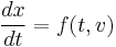
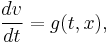
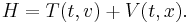
where f and g are given functions. Here, x and v may be either scalars or vectors. The equations of motion in Hamiltonian mechanics take this form if the Hamiltonian is of the form
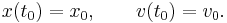
The differential equations are to be solved with the initial condition
The method
The semi-implicit Euler method produces an approximate discrete solution by iterating
![\begin{align}
v_{n%2B1} &= v_n %2B g(t_n, x_n) \, \Delta t\\[0.3em]
x_{n%2B1} &= x_n %2B f(t_n, v_{n%2B1}) \, \Delta t
\end{align}](/2012-wikipedia_en_all_nopic_01_2012/I/32f3866cc55a6a3ae99ed5a82ef5548d.png)
where Δt is the time step and tn = t0 + nΔt is the time after n steps.
The difference with the standard Euler method is that the semi-implicit Euler method uses vn+1 in the equation for xn+1, while the Euler method uses vn.
Applying the method with negative time step to the computation of  from
from  and rearranging leads to the second variant of the semi-implicit Euler method
![\begin{align}
x_{n%2B1} &= x_n %2B f(t_n, v_n) \, \Delta t\\[0.3em]
v_{n%2B1} &= v_n %2B g(t_n, x_{n%2B1}) \, \Delta t
\end{align}](/2012-wikipedia_en_all_nopic_01_2012/I/1d65b0b00cfe135ec0ab8100747acf0e.png)
which has similar properties.
The semi-implicit Euler is a first-order integrator, just as the standard Euler method. This means that it commits a global error of the order of Δt. However, the semi-implicit Euler method is a symplectic integrator, unlike the standard method. As a consequence, the semi-implicit Euler method almost conserves the energy (when the Hamiltonian is time-independent). Often, the energy increases steadily when the standard Euler method is applied, making it far less accurate.
Alternating between the two variants of the semi-implicit Euler method leads in one simplification to the Störmer-Verlet integration and in a slightly different simplification to the leapfrog integration, increasing both the order of the error and the order of preservation of energy.[1]
Example
The motion of a spring satisfying Hooke's law is given by
![\begin{align}
\frac{dx}{dt} &= v(t)\\[0.2em]
\frac{dv}{dt} &= -\frac{k}{m}\,x=-\omega^2\,x.
\end{align}](/2012-wikipedia_en_all_nopic_01_2012/I/bb7f669d0c9e9cb0bee8a9e5a64566dc.png)
The semi-implicit Euler for this equation is
![\begin{align}
v_{n%2B1} &= v_n - \omega^2\,x_n\,\Delta t \\[0.2em]
x_{n%2B1} &= x_n %2B v_{n%2B1} \,\Delta t.
\end{align}](/2012-wikipedia_en_all_nopic_01_2012/I/6d46816361d7e2cfe07e4eee5801c289.png)
The iteration preserves the modified energy functional  exactly, leading to stable periodic orbits that deviate by
  from the exact orbits. The exact circular frequency
  increases in the numerical approximation by a factor of
  .
.
References
- ^ Hairer, Ernst; Lubich, Christian; Wanner, Gerhard (2003). "Geometric numerical integration illustrated by the Störmer/Verlet method". Acta Numerica 12: 399–450. doi:10.1017/S0962492902000144. http://citeseerx.ist.psu.edu/viewdoc/summary?doi=10.1.1.7.7106.
- Giordano, Nicholas J.; Hisao Nakanishi (July 2005). Computational Physics (2nd edition ed.). Benjamin Cummings. ISBN 0-1314-6990-8.
- MacDonald, James. "The Euler-Cromer method". University of Delaware. http://www.physics.udel.edu/~jim/Ordinary%20Differential%20Equations/Euler-Cromer%20Method.htm. Retrieved 2007-03-03.
- Vesely, Franz J. (2001). Computational Physics: An Introduction (2nd edition ed.). Springer. pp. page 117. ISBN 978-0-306-46631-1.
|
|||||||||||